Sound localisation model

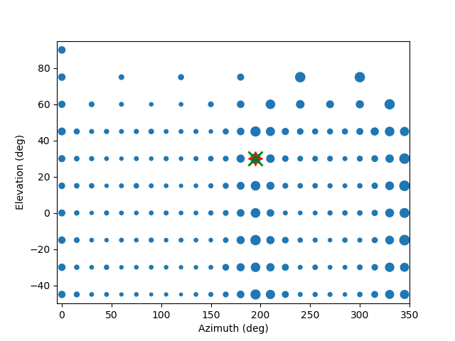
Example demonstrating the use of many features of Brian hears, including HRTFs, restructuring filters and integration with Brian. Implements a simplified version of the “ideal” sound localisation model from Goodman and Brette (2010).

The sound is played at a particular spatial location (indicated on the final plot by a red +). Each location has a corresponding assembly of neurons, whose summed firing rates give the sizes of the blue circles in the plot. The most strongly responding assembly is indicated by the green x, which is the estimate of the location by the model.

Note that you will need to download the IRCAM_LISTEN database and set the IRCAM_LISTEN environment variable to point to the location where you saved it.

Reference:

Goodman DFM, Brette R (2010). Spike-timing-based computation in sound localization. PLoS Comput. Biol. 6(11).

from brian2 import *
from brian2hears import *

# Download the IRCAM database, and replace this filename with the location
# you downloaded it to
hrtfdb = IRCAM_LISTEN()
subject = hrtfdb.subjects[0]
hrtfset = hrtfdb.load_subject(subject)
# This gives the number of spatial locations in the set of HRTFs
num_indices = hrtfset.num_indices
# Choose a random location for the sound to come from
index = randint(hrtfset.num_indices)
# A sound to test the model with
sound = Sound.whitenoise(500*ms)
# This is the specific HRTF for the chosen location
hrtf = hrtfset.hrtf[index]
# We apply the chosen HRTF to the sound, the output has 2 channels
hrtf_fb = hrtf.filterbank(sound)
# We swap these channels (equivalent to swapping the channels in the
# subsequent filters, but simpler to do it with the inputs)
swapped_channels = RestructureFilterbank(hrtf_fb, indexmapping=[1, 0])
# Now we apply all of the possible pairs of HRTFs in the set to these
# swapped channels, which means repeating them num_indices times first
hrtfset_fb = hrtfset.filterbank(Repeat(swapped_channels, num_indices))
# Now we apply cochlear filtering (logically, this comes before the HRTF
# filtering, but since convolution is commutative it is more efficient to
# do the cochlear filtering afterwards
cfmin, cfmax, cfN = 150*Hz, 5*kHz, 40
cf = erbspace(cfmin, cfmax, cfN)
# We repeat each of the HRTFSet filterbank channels cfN times, so that
# for each location we will apply each possible cochlear frequency
gfb = Gammatone(Repeat(hrtfset_fb, cfN),
                tile(cf, hrtfset_fb.nchannels))
# Half wave rectification and compression
cochlea = FunctionFilterbank(gfb, lambda x:15*clip(x, 0, Inf)**(1.0/3.0))
# Leaky integrate and fire neuron model
eqs = '''
dV/dt = (I-V)/(1*ms)+0.1*xi/(0.5*ms)**.5 : 1 (unless refractory)
I : 1
'''
G = FilterbankGroup(cochlea, 'I', eqs, reset='V=0', threshold='V>1', refractory=5*ms, method='Euler')
# The coincidence detector (cd) neurons
cd = NeuronGroup(num_indices*cfN, eqs, reset='V=0', threshold='V>1', refractory=1*ms, method='Euler', dt=G.dt[:])
# Each CD neuron receives precisely two inputs, one from the left ear and
# one from the right, for each location and each cochlear frequency
C = Synapses(G, cd, on_pre='V += 0.5', dt=G.dt[:])
C.connect(j='i', skip_if_invalid=True)
C.connect(j='i-num_indices*cfN', skip_if_invalid=True)
# We want to just count the number of CD spikes
counter = SpikeMonitor(cd, record=False)
# Run the simulation, giving a report on how long it will take as we run
run(sound.duration, report='stderr')
# We take the array of counts, and reshape them into a 2D array which we sum
# across frequencies to get the spike count of each location-specific assembly
count = counter.count[:].copy()
count.shape = (num_indices, cfN)
count = sum(count, axis=1)
count = array(count, dtype=float)/amax(count)
# Our guess of the location is the index of the strongest firing assembly
index_guess = argmax(count)
# Now we plot the output, using the coordinates of the HRTFSet
coords = hrtfset.coordinates
azim, elev = coords['azim'], coords['elev']
scatter(azim, elev, 100*count)
plot([azim[index]], [elev[index]], '+r', ms=15, mew=2)
plot([azim[index_guess]], [elev[index_guess]], 'xg', ms=15, mew=2)
xlabel('Azimuth (deg)')
ylabel('Elevation (deg)')
xlim(-5, 350)
ylim(-50, 95)
show()